3D-Printer and Your Coffee Grinder

Two weeks ago I acquired a 3D printer; specifically the Printrbot Simple Metal Kit and, after some warranty help, it’s printing well. The first thing I printed was the fan shroud for the 3D printer itself, as recommended by Printrbot, but the next things were for my own design. I printed a set of three sieves, to fulfill my long-time dream of quantifying the performance of coffee mills.

For those of you who read my coffee blog posts years ago, I was frustrated because nobody quantifies the grind performance. Vendors and coffee pundits are happy to talk about the merits of a conical burr grinder or fret about the cheap blade grinder you got from your lost year with Gevalia. Quantifying grinder performance should be pretty straightforward. Take a set of sieves and sort the grinds by size, the more consistent grinders will produce more grounds in a narrow range of sizes. Spoiler: I have only measured my whirling blade grinder so far, not my Capresso burr grinder or any of the commercial grinders.

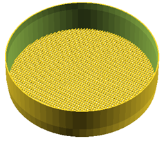
The printed sieves are just cylinders with a printed mesh bottom. They don’t stack well, since I used too little taper. My finest one had holes so small that it plugged with the finest coffee dust, so there is more to do in the sieve design. Nevertheless, I started with the mesh from Thingiverse, and added 15 mm of wall height. When I get a version of these that stacks I’ll post the design to the Thingiverse too.

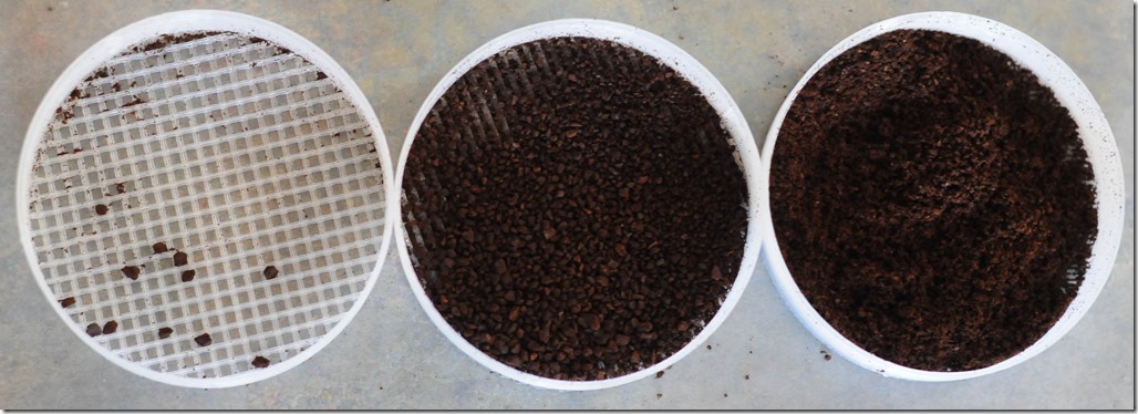
I arranged the sieves in a stack and shook. The sieves clogged almost immediately, so I took a small brush and worked the from the top layer down until I had good separation.

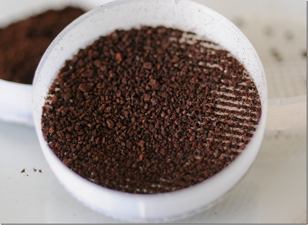
The results, in the following picture, show that almost no particles were larger than my largest mesh, less than half were larger than my medium mesh, and the rest were larger than my fine mesh.

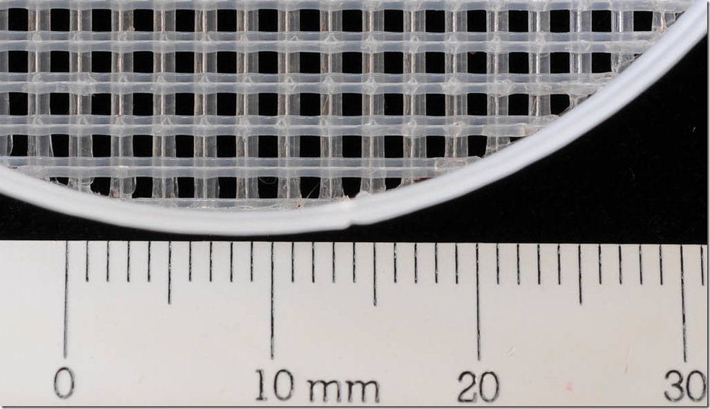
So what are the mesh sizes? I took macro photos of the meshes and then measured them optically—you know, counted pixels. The composite photo below shows the basic idea, and below that is a zoomed-in version of the medium sieve.

The medium sieve is made from “threads”, where each “thread” is two passes with the extruder head. It should be possible to do a single extruder path, but I have not yet tuned the OpenSCAD file to get a consistent result.

Mesh	Cell Diagonal	Coffee	Percent
Coarse	2.5 mm	<0.1 g	0%
Medium	1.4 mm	1.0 g	28%
Fine	0.48 mm	2.6 g	72%
	fall through	<0.1 g	0%

Whether grind consistency can actually be identified by a taster in a blind test is an open, and wonderful, question. Happy brewing!

Coffee to Water Ratio

A friend of mine (thanks Marc!) forwarded the linked article to me last week.  While it is more of a coffee tease sort of thing than anything else, it just so happens that the article discusses the coffee/water ratio used by some of these gluttons.  You’ll be surprised how modest my recipe looks.

New York is Finally Taking Its Coffee Seriously, NY Times, March 9, 2010.

Coffee: Model Fitting Goodness

You have seen the response function contours through the stationary point, and you have seen the 3D response function visualizations. You may recall that I have two competing models, one is derived from the experimental data design for the response surface, and the other is all that data and the screening results too. Is either model any good? Which one is better?

First, a quick review of the model:

q = b₀T² + b₁t² + b₂r² + b₃Tt + b₄tr + b₅Tr + b₆T + b₇t + b₈r + b₉

Fitting produces numbers for all those coefficients, b₀, b₁, etc. Look at the goodness of individual coefficients in the following table. The more asterisks in the significance column, the better the coefficient corresponds to the data. Notice that the “all data” model has an overall terrible goodness, with the residual standard error of 0.7, compared to the residual error of 0.358 for the RSO data only.

	All Data			RSO Data Only
Std Error	0.749			0.358
	Estimate	Std. Error	Signif.	Estimate	Std. Error	Signif.
(Intercept)	3.344	0.3963	***	3.6667	0.2064	***
temp	-0.355	0.2369		-0.4375	0.1264	*
time	0.235	0.2369		0.0375	0.1264
cwrat	0.4	0.2369		0.275	0.1264	.
temp:time	-0.5	0.2901		-0.75	0.1788	**
temp:cwrat	0.02	0.2901		-0.375	0.1788	.
time:cwrat	0.09	0.2901		-0.075	0.1788
temp^2	-0.401	0.3592		-0.6833	0.1861	*
time^2	-0.201	0.3592		-0.4833	0.1861	*
cwrat^2	0.174	0.3592		-0.1083	0.1861
Significance codes: 0 ‘***’ 0.001 ‘**’ 0.01 ‘*’ 0.05 ‘.’ 0.1 ‘ ‘ 1

The two graphs below show the quantile normal plots for the residuals from each model. The all-data model looks more systematically erroneous than the RSM data only. The systematic error suggests that the choice of model is not particularly good. Furthermore, it suggests that the estimates of F-statistic should be considered hesitantly, as F-statistics are calculated by assuming normally distributed independent errors.

With hesitation then, let’s examine the F-statistic for these models. The RSO data model produces an F-statistic of 6.4, well above the Box, Hunter, and Hunter criterion that the F-statistic exceeds 4. On the other hand, the all data model’s F-statistic is a miserly value of 1.

	All Data	RSO Data Only
Degrees of Freedom	9	5
Residual Standard Error	0.749	0.358
F-statistic	1.06	6.43

In conclusion, I get a better fit—to the indicated model—using only some of the data. This is, frankly, an indictment of the model. Anyone can carefully select data to produce a good fit to a model, and the fact that I have done so may be considered a round condemnation of my objectivity. I may reconsider the model, and attempt to drop the least important terms while adding either a three-way interaction or two-way involving squares. Perhaps more creative math will be required.

Coffee: Visualizing the Response Function

I have been calling my 3D response function a “surface”—which is linguistically feckless at best. Of course, I have some company, the immortal Box, Hunter, and Hunter call the experiment design a response surface method. So note carefully, the response function is not a surface, it completely fills a volume.

Naturally, this is hard to visualize. The contour plots are slices through the response space, but I really have a hard time inferring what my coffee quality function is telling me. Better visualization to the rescue.

First, put the contour plots together into slices, using just the shaded parts and not the lines. Note that these cuts run through the center of the design point, and not the stationary point.

This is still quite difficult to interpret. The blue and green corners of the areas are clearly to be avoided, while the red-tinted areas near the top are to be embraced. Red, in all these plots, is a higher value of q than blue. The weird little balls are the points on the steepest ascent experiment path. Their radius corresponds to their predicted q values. Tufte, of course, would have a fit; clearly the volume should be proportional to the indicated variable.

Those planar cuts are nice to look at, but we can do even better. Add “isosurfaces”—these are surfaces that lie on constant values of q. In two dimensions a topo map shows lines of constant elevation. For 3D data, the lines become surfaces. In the following figure I’ve kept the horizontal cut, and added isosurfaces. The big black line shows the steepest ascent.

This is getting useful. To make a good cup of coffee, you want to be somewhere in the red cup on the upper-left-front corner. The zone is not enormous. To more clearly visualize this, here is the same concept from a few different angles.

So, here we are, and I still don’t have a good idea what the response function looks like outside the design space. Clearly there is a region in the middle which is relatively high quality, and it appears that higher C/W ratios are favored.

Finally, to get a solid sense of the response function I thought it would be helpful to zoom out. The next graph shows the response function in extrapolated over a much wider range.

The little box in the middle is the design space. In this case there are four isosurfaces drawn, for q=1,2,3,4. With this visualization you can clearly see the shapes represented by the response function. I’m sure that the function is a poor representation of truth in the regions far from the design space. Nevertheless, this diagram is more helpful to me than any other, as I can see there is clearly a cup-shaped region in which my coffee should be really awesome. The region is surprisingly narrow over C/W ratio, time, and temperature. A poor-man’s sensitivity analysis.

All the previous analysis has been on the response surfaces for the RSO data set only, that is, I left out the original data from the screening experiment. If I include the alternate data the fit remains qualitatively similar in that there is a tasty region in the upper left hand part of the original design space. However, the rest seems very different. There is now a saddle point, and more of the design space is better than before. Now, too, the steepest ascent path points toward increasing C/W ratio and decreasing temperature. Unlike the previous fit, though, there is substantial decrease in time inferred. Furthermore, this surface admits quality values in excess of 5. The upper isosurface is q = 5.

Resources

On the off chance you’re wondering how I made these really cool plots…

Analysis of the experiment and fitting of the response model to the data was accomplished in the wonderful language R. I couldn’t find any way to do cut-planes in R, and in any case am not terribly good with it. So I used Python(x,y) with the Enthought Tool Suite, in particular the mlab and Mayavi interfaces. Many, many thanks to the good people of the Pythonic world, and especially Enthought, for the quality product they have created. Who needs Matlab anyway?

My source code is available upon request.

Coffee: Analysis & Results of the Response Surface

I have executed the experiment design discussed Coffee: Design of the Experiments (Part 2: RSO). This “response surface method” experiment design is carefully crafted to provide the data necessary to fit a formula of the form

q = b₀T² + b₁t² + b₂r² + b₃Tt _{+ b4tr + b5Tr + b6T + b7t + b8r + b9}

This model describes quadratic terms (T², t², r²), main effects (T, t, r), and first-order interactions (Tt, tr, Tr). The model basically assumes that quality is locally curved or locally linear, but not an undulating surface. This assumption of local smoothness is a good one in this case—were it not the experience of buying a cup of a coffee would be a dangerous gamble where small changes made by the brewer resulted in big changes in our cup.

Some possible findings in our analysis

• There is a maximum value of q at some point in the design space, whose approximate location we can find with the preceding method.
• There is a maximum value of q at the edge of the design space, that is, we might find that the best q occurs at some maximum value of concentration (a face of the design cube), or even, for example, the maximum value of concentration and temperature (an edge of the design cube), or a maximum of all the values (a corner of the design cube).
• Some variables don’t matter, and the entire experience is governed by only one variable—indeed the screening experiment hinted at this outcome.

If the optimum is inside the design space, then I know immediately how to brew the best cup of coffee—within some amount of error. If the optimum is outside the design space, at least I know which experimental trend to pursue. Namely, new experiments are positioned along the path of most rapid ascent, or a new design cube is positioned outside the current design cube, with the center moved along the path of most rapid ascent.

Results

The following three graphs show slices through the response surface fit to the experiments. The slices are positioned so that they intersect the “stationary point”. If there is a local maximum, then it is the stationary point; the plots then display the local sensitivity around that stationary point. The quadratic fit can also produce saddle-shaped responses, in which case the center of the saddle is a stationary point.

Note that these plots are all based on the fit to just the response surface design. A different fit is obtained by including the data from the screening results.

The graphs all work in “coded variables”, that is, they are all adjusted so that the values lie between -1 and 1. It is necessary to decipher these values into measureable numbers, which the following equations do. The coded value is indicated with a c subscript.

Time t_c = 1.35log₁₀(t) – 2.35

Temperature T_c = 0.1(T – 195)

C/W Ratio r_c = 50(r – 0.055)

These equations are easily inverted, though below I provide uncoded (normal) values for the points in the steepest ascent.

The fitted space suggests that water temperature is important—certainly more important than the screening experiment suggested. However, my cup quality actually improves as the temperature declines. Almost all the brewing words I’ve read, including the latest Consumer Reports, harp on the importance of getting water hot enough. My experiment suggests that modulating extraction duration and C/W ratio are at least as important.

Steepest Ascent

The response surface methodology encourages further experiment design. Starting from the stationary point, you can follow the path of steepest ascent to move toward ever better quality—at least in theory. To my surprise, this worked for a one-trial qualitative test; more on that later. The steepest ascent predicted using the fit to just the RSO data is shown in the next table. Note that the concentration of coffee is quickly leaves the design space, which was limited to concentrations less than 0.075.

Steepest (RSO only)
Time [sec]	Coffee [g]	Water [fl oz]	Temp [F]	C/W Ratio [g/ml]	Predicted Q
55	22.3	13.7	195	0.055	3.7
69	22.3	12.1	192	0.062	3.9
90	22.3	10.7	190	0.071	4.1
116	22.3	9.5	187	0.079	4.3
148	22.3	8.6	185	0.088	4.4
188	22.3	7.8	183	0.096	4.6
238	22.3	7.2	181	0.105	4.7
301	22.3	6.6	179	0.114	4.8
380	22.3	6.2	177	0.123	4.9
479	22.3	5.7	175	0.131	5.0
601	22.3	5.4	173	0.140	5.0

A similar fit using all the available data produced the steepest ascent trials in the next table. It is, perhaps, less believable since the quality values rise in excess of 10.

Steepest (RSO + Screening)
Time [sec]	Coffee [g]	Water [fl oz]	Temp [F]	C/W Ratio [g/ml]	Predicted Q
55	22.3	13.7	195	0.055	3.3
78	22.3	12.0	193	0.063	3.7
105	22.3	10.4	192	0.072	4.0
132	22.3	9.2	191	0.082	4.5
161	22.3	8.2	190	0.092	5.1
192	22.3	7.4	190	0.102	5.7
226	22.3	6.8	190	0.112	6.4
264	22.3	6.2	189	0.121	7.2
307	22.3	5.7	189	0.131	8.1
355	22.3	5.3	189	0.141	9.1
409	22.3	5.0	188	0.151	10.2

Despite the implausibility, I conducted a trial of the 3^rd experiment in the combined table, that is, 105 seconds extraction at 192 F for a 0.072 concentration coffee. My results:

“Quality = 4.2. Toasted marshmallow flavor! Aroma is rich and without char. Acid and bitter are nicely balanced in the first sip but the bitter dominates the aftertaste.”

The quality agreement (and I really didn’t peak) is unexpectedly close—4.2 instead 4. Furthermore, there I was genuinely surprised at entirely new flavors. It really was a great cup of coffee. Damned strong though.

For comparison, the contour plots produced by the fit to the RSO data and the screening data are shown next.

A future post will discuss the goodness of fit, and whether the models are meaningful. For the present, rest assured that predicting a quality of 4 and measuring the same convinces me that the results are useful.

Data

The actual data, along with my notes at the time, is shown in the following table.

Coffee [g]	Water [fl oz]	C/W [g/ml]	Time [sec]	Temp [F]	Trial Order	Q	Date	Comment
22.8	14.0	0.055	300	205	1	1.5	2/20/2009	Not good. Bitter flavor with simple aroma. Too bitter
22.8	22.0	0.035	55	205	2	2.5	2/23/2009	Simple flavor with muted cemplexity. Aroma and flavor dominated by char. Neither too bitter nor too acid. Not balanced though.
22.8	14.0	0.055	10	205	3	2.5	2/24/2009	Too bitter. Aroma fairly simple. Mouth feel too watery. Little acidity, poorly balanced between acid and bitter.
22.8	10.3	0.075	55	185	4	4	2/25/2009	Aroma is excellent w/ complex interesting smells. There is some crema. Nicely acidic and reasonably balanced w/ bitter.
22.8	14.0	0.055	55	195	5	3.5	3/2/2009	Acid-bitter balance too heavy on bitter side. Nice crema and nice aroma. Rich mouth feel.
22.8	22.0	0.035	10	195	6	3	3/3/2009	Moderately well balanced. Aroma is simple. Mouth feel watery.
22.8	14.0	0.055	55	195	7	4	3/4/2009	Well balnced w/ good aroma. A little too bitter, but not unpleasant.
22.8	10.3	0.075	10	195	8	3.5	3/5/2009	Aroma somewhat simple. Flavor strong or even rich. Too bitter overall and acid/bitter balance poor.
22.8	14.0	0.055	10	185	9	2	3/6/2009	Bitter simple flavor without much acid. Aroma is farily good but not as rich as I like.
22.8	10.3	0.075	300	195	10	3	3/9/2009	Smelled bitter. Taste moderately well balanced with a little too much bitter. Rich feel.
22.8	22.0	0.035	300	195	11	2.8	3/10/2009	Watery. Yet implanaced toward bitter. Flavor is well-bodied and aroma good.
22.8	10.3	0.075	55	205	12	2.5	3/11/2009	Burned and charred taste. Too bitter while also being nicely acidic. Not well balanced. Aroma dominated by char.
22.8	22.0	0.035	55	185	13	2.5	3/12/2009	Aroma dominated by char and relatively uninteresting. Taste is poorly balanced–too bitter. Strong flavor.
22.8	14.0	0.055	300	185	14	4	3/16/2009	Well balanced and nicely aromatic. A little bitter on the finish.
22.8	14.0	0.055	55	195	15	3.5	3/17/2009	Bitter flavor with weak mouth feel and low complexity. Aroma nicely balanced though.

Coffee: Considering Cold Extraction

I won’t start the cold extraction experiments until I finish the response surface set, and possibly until I perform some local optimization using the RSO outcome. To warm up, paradoxically, here are some thoughts on cold extraction.

The basic process, everywhere I’ve read about it, is to put grounds in room temperature water for a long time—overnight for example—and then filter or decant the extract into storage. The extract is generally much stronger than regular coffee, and so to serve it you dilute it with hot water.

Naturally, you can buy expensive equipment to help this process, or you can use a French press. I imagine that decanting through your drip pot’s filter cage would work well too.

Economics

The premier advocate of the method would appear to be Toddy Products. They recommend extracting one pound of beans in 9 cups water, then reconstituting the coffee with 3:1 hot water to coffee extract. I’m guessing that you get about 8 cups of extract, and in turn 32 cups of coffee. I believe that Toddy is talking about 8 fl oz cups, though in the world of coffee you can never be certain. In any case, 1 lb of coffee to about 32 cups of water corresponds to a C/W ratio of 0.060 g/ml. This compares quite reasonably with the C/W ratio used in hot brewing. Recall that in my experimental set-up I use ratios between 0.035 and 0.075 g/ml.

Another site recommends using 1 gallon (16 cups) of water with 1 lb of coffee. All the other sites I examined suggest similar ratios of approximately 0.060 g/ml.

Grind Size

Recommended grind size is coarse, though it appears the reason is to allow easy filtering. Since extraction time is 6 to 12 hours, depending on reference, I suspect that what dominates the extraction process is the solubility of various compounds at room temperature, rather than the diffusion of those chemicals from the beans. Any old grinder is probably fine, and variation in the particle size is probably irrelevant.

Predictions

I believe this process will make an insipid cup of coffee. It is recommended by some because it produced lower acidity and less bitterness. Translation: less flavor. Terroir Coffee asserts that the “resulting cup is light bodied and bland since all acidity and many aromatics, which require hot water for the right chemical reactions, are never formed.” Not inspiring. Of course, I didn’t think brewing coffee had much to do with chemical reactions as with dissolution…

The process offers great convenience in that you can brew just once for two weeks’ coffee. Furthermore, it should be palatable to people who like weak coffee. The strength of the cup can be easily changed to suit the members of your party.

Coffee: Design of the Experiments (Part 2: RSO)

In Review

The results of my 4-trial fractional factorial experiment (main effects) showed that extraction time is the most important variable, and that temperature and C/W ratio are less important. In the interest of completeness this experiment will not simply vary extraction time, but rather seek to efficiently find the maximum.

Lessons from the Screening Experiment

I am accustomed to making my coffee with about 22 fluid ounces of water, which makes two nice cups for my morning. During the screening I used 22 fl oz as a baseline, and increased or decreased the amount of coffee accordingly. The result was that some experiments required 48.8 g of coffee. You can’t possibly imagine how much coffee that is. It almost completely fills a coffee cup with just the beans!

In subsequent experiments I will limit the amount of coffee beans to something more modest, perhaps about 20 g, and vary the amount of water. With this more cautious approach I may live to see the final results.

The Design

NIST offered three designs for response surface objective (RSO) experiments. Specifically there are two interpretations of the Box-Wilson central composite design, each of which requires 20 total runs. An alternative design reduces the number of experiments to 15, which is the reason I chose it.

Specifically, the Box-Behnken design provides an RSO approach for 3 factors in 15 experiments. That is the same number I originally suggested through my naïve approach, but without all the baggage. Effectively, my original 5 values for each factor get reduced to three, and those are shuffled about in a way that is well-suited to estimating their effects. In my case, the specific experiments would be:

Response Surface Objective
	Actual Values			Statistics Jargon
Trial	r (g/ml)	t (sec)	T (F)	R	T	T
1	0.035	10	195	-1	-1	0
2	0.075	10	195	+1	-1	0
3	0.035	300	195	-1	+1	0
4	0.075	300	195	+1	+1	0
5	0.035	55	185	-1	0	-1
6	0.075	55	185	+1	0	-1
7	0.035	55	205	-1	0	+1
8	0.075	55	205	+1	0	+1
9	0.055	10	185	0	-1	-1
10	0.055	300	185	0	+1	-1
11	0.055	10	205	0	-1	+1
12	0.055	300	205	0	+1	+1
13, 14, 15	0.055	55	195	0	0	0

This set will take me about three weeks. With luck by the time you read this I will have trickled out previous articles, and you will have results in two weeks or less. Sorry for the suspense.

Oh yes, I’m interested in other people’s Q functions too, so if you want to run my exact experiments, please post your data and I will post your results. Public or anonymous, at your discretion.

Coffee: The Detestitron

Please, when you are shopping for a grinder, don’t believe anything you hear (except what I tell you…). A blade grinder is probably as good a grinder as you want to afford. Don’t presume that a burr grinder will automatically produce a more consistent grind. Take, for example, my manual burr machine. Compare the grind consistencies from my cheapo blade grinder with my burr grinder in the following picture. Neither is “consistent”, and the variation from the burr grinder goes from about 4 mm to dust. The blade grinder produces 1 mm to dust. Neither appears to produce a dominant particle.

You may want to cover your children’s eyes; even a brief look at this grinder could give them nightmares.

Detestitron is a heavily modified portable burr grinder. It was about $20, but it uses conical ceramic burrs and is quite ingeniously designed. The modifications I made to the original grinder maintain concentricity between the inner and outer cones, and facilitate holding the cursed thing to the table while turning the crank. The grind consistency, for all that, did not actually improve noticeably.

The Detestitron’s grind axle is centered in ball bearings. The original shaft was extended with a small brass rod, brazed on. The bottom bearing is fixed in an aluminum bar, which is in turn screwed to the chassis. Note that the center cone is not perfectly round, and so this keeps the grinder very stable—but it is not really centered.

The burrs are basically the same as you would see on a pepper mill, but much larger. There is a screw-like mechanism to force the beans into the narrow grinding slot.

Detestitron’s fundamental problem is that the length of the surfaces over which there is a consistent separation is very short—the coarser the grind, the shorter the overlapping length. I believe that any grinder with similar burrs would produce similar results. There are other designs, but they seem to start at about $200. Did I mention donations are welcome?

Coffee: Analysis & Results of the Main Effects Study

I have conducted the trials in the following table.

	Actual Values			Statistics Jargon
Trial	r (g/ml)	t (sec)	T (F)	r	t	T	Q
1	0.035	10	205	-1	-1	+1	2.5
2	0.075	10	185	+1	-1	-1	3
3	0.035	300	185	-1	+1	-1	4
4	0.075	300	205	+1	+1	+1	4.1

This study is a 2-factor partial factorial design, indicated as 2^3-1. The good people who write for Wikipedia tell me that this experiment design gives “main effects” but those may be confounded with two-factor interactions. Indeed, there is some reason to be concerned for the simple quality function evaluation in this situation—for example, I worry that row 1 and row 2 could easily produce similar effects. C/W is lower in 1, but the temperature is higher, so extraction should be similar to a higher ratio with lower temperature. In any case, if the result is not revealing, the experiment may be augmented with the remaining 4 cases in the factorial design.

The main effects plot shows how each parameter influences the result, though recognize that interactions may be masking main effects. The main effects plot for this experiment is shown below. From this it would appear that extraction time is the most sensitive parameter—to me a surprising observation. I had certainly expected the coffee/water ratio (cwrat) to be the dominant variable, but here it does not appear to be so. The negative correlation with temperature is very surprising, and indeed I am skeptical. Still, the variation appears to be quite small, and is likely due to two-factor interactions.

I would be inclined to fix the temperature and the C/W ratio at their midpoints, and vary the time alone; however, I believe the response hypersurface is more complex. I shall press forward with the response surface methodology on all three variables.

In case you want to see my data.

Trial Order	Q	Date	Comment
1	2.5	2/16/09	Dishwatery taste and aroma. Very simple palate with almost no mouth feel. Equivalent to mediocre drip.
2	3	2/17/09	Not very aromatic and too simple. Has nice bitterness and some acidity but not well balanced between them.
3	4	2/18/09	Mildly aromatic. Good mouth feel with acid/bitter well balanced. Slight char flavor.
4	4.1	2/19/09	Too bitter. The aroma is marvelous being very rich and tantalizing. Mouth feel is creamy. If bitterness where attenuated this would be sublime.

I wasn’t going to use fractions, but I decided I needed them. Note that trial 4 was assigned a quality of 4.1, which is really a note saying that this was a little bit better than trial 3, but not much.

Coffee Design of Experiments (Part 1: Screening)

I will invoke a variety of principals from experiment design methods. The truth is, though, that I’m self-taught in experiment design. It is altogether probable that there are better ways of conducting this experiment which my ignorance has hidden from me. I’m open to suggestions!

Quick Review

The variables in control are temperature t, extraction time T, and coffee-to-water ratio (by weight) r. Each of these will be considered over a domain of 5 values. Temperature and coffee-to-water ratio are linearly divided into 5 steps between their minimum and maximum values, which I selected based on published coffee brewing advice. Extraction time is divided logarithmically over its domain, since my intuition is that extraction is an approximately logarithmic process in time.

Linear Uncorrelated Approach

I might assume that t, T, and r are uncorrelated and independent. Then, without assuming that Q is linear in t, T, or r, I could easily conduct the following experiments (if the mathese bothers you, skip ahead to the text):

• T = 195 F, t = 55 seconds, r =
  (0.035, 0.045, 0.055, 0.065, 0.075) g/ml
• T = 195 F, t = (10, 23, 55, 128, 300) seconds, r = r_max = argmax_r
  Q(r, T = 195, t = 55)
• T = (185, 190, 195, 200, 205) F, t = t_max = argmax_t Q(r = r_max, T = 195, t)

In English, first find the best point by finding the optimum coffee-to-water ratio for a fixed extraction period and temperature. My experience suggests that the ratio is likely to be one of the more sensitive parameters, so sweeping this first should provide good insight. Then, using that optimum C/W ratio, sweep the extraction time to find the best duration. Finally, sweep the temperature.

Really, this is a sort of bastardized gradient search. It doesn’t account for correlation among parameters. For example, you might imagine that a very high C/W ratio combined with a short extraction time would produce a very different flavor than the same high C/W ratio and a long extraction time. In fact, one might be delicious and the other dreadful. The proposed methodology, however, would not reveal that condition.

Another problem is that it really isn’t safe to assume only 15 trials would be required. The quality function (my enjoyment) is likely to be quite subjective and quite variable—I’ll assume for argument that it is also Gaussian. Q can take integer values from 1 to 5, and it is quite reasonable to assume that my variability has a standard deviation is 1.5 or so. To know the actual quality accurate to a single value of Q with 95% certainty requires the standard deviation to be about 0.25. We can reduce the standard deviation of the estimated Q by averaging multiple experiments. How many? (1.5/0.25)² = 25. Now the original 15 trials have turned into 15×25 = 375, and at 1 experiment per day pushed the answer a year into the future.

A savvy person might ask if there is a way to find an equally good answer with fewer experiments or if there is a better way to arrange those 375 experiments to get more broadly useful answers.

NIST provides a sublime search tree for selecting an experiment design, and it is clear that what I’ve outlined is best served by a response surface objective (RSO) on 3 factors, or possibly a main effects design first, followed by a response surface objective on 2 or 3 factors, or even a simple 1-factor search.

While I expect to consider the RSO approach in terms of number of experiments, and then examine a screen+RSO approach to see if there is a design which offers possibly reduced number of experiments. The Box-Behnken design for RSO in 3-factors requires a paltry 15 experiments. Still, that is three weeks away, and I would prefer to have some data to work with sooner.

The screening test is much smaller, and perhaps worthwhile in that the data can be included in the RSO experiment, even though not strictly required. For my 3-factor system the Level III screening design requires a modest 4 runs. This would be small enough that I could even do two trials of each, which would be of great help in reducing my variability. The experiments are listed in the following table.

Screening Design
	Actual Values			Statistics Jargon
Trial	r (g/ml)	t (sec)	T (F)	r	t	T
1	0.035	10	205	-1	-1	+1
2	0.075	10	185	+1	-1	-1
3	0.035	300	185	-1	+1	-1
4	0.075	300	205	+1	+1	+1

If I Had a Grinder

The other major effect that I would like to measure is grind size, predicated on substantially uniform product. My grinder doesn’t do it. Consider, though, the 4-factor version of this same exercise. The four-factor RSO requires 33, 46, or 52 experiments, depending on the method. The four-factor screen requires 8 experiments. Even if the screening doesn’t reduce the number of factors substantially, the experiment is tractable at 41 trials. Of course all this assumes Q has tolerable variance.

If you donate the grinder, I’ll do the experiments…